FluxFlow

Ground-to-space image reconstruction

FluxFlow

Conservative Flow-Matching forAstronomical Image Super-Resolution

Reconstruct finer structure from DESI observations while keeping source flux and measurement consistency in view.

  • Liuzhuozheng Li1
  • Gengjia Chang2
  • Jun Liu2
  • Ziying Gu1
  • 1The University of Tokyo
  • 2I2WM
  • 3Shanghai Astronomical Observatory (SHAO)
  • 4Tohoku University
  • 5RIKEN

* Equal contribution  ·  ◆ Corresponding author

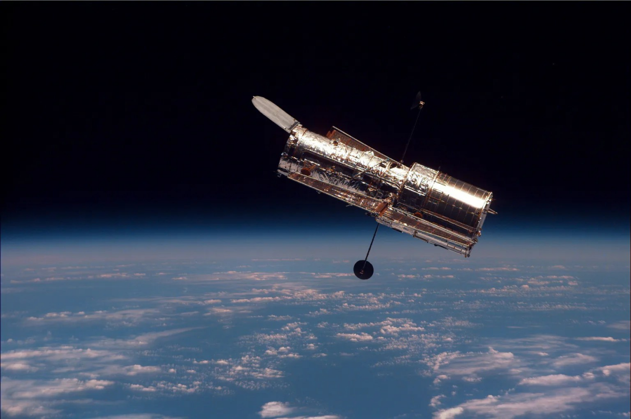
Hubble Space Telescope above Earth's clouds and atmospheric limb. NASA photograph supplied in the website requirements.

From ground to space

A clearer view above the atmosphere

Moving air blurs the light reaching a ground-based telescope. Hubble observes above this turbulent layer.

The challenge is to recover useful structure from the ground image without adding unsupported sources.

Meet the two observations

View the photograph ↗Hubble above Earth · NASA

The observations

Two views of the same sky

DESI records the ground view. HST provides a matched, higher-resolution reference.

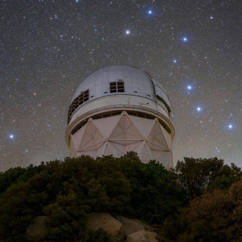
Ground-based observatory shown in the paper's instrument figure.

The input · from the ground

DESI Legacy Imaging Surveys

An i-band cutout is the measured input. Each 128 × 128 patch is paired with the same sky region in HST.

Observation used here
Single-band i image
Input cutout
128 × 128 pixels

Observatory photograph from the paper's instrument figure; the imaging surveys combine observations from multiple telescopes.

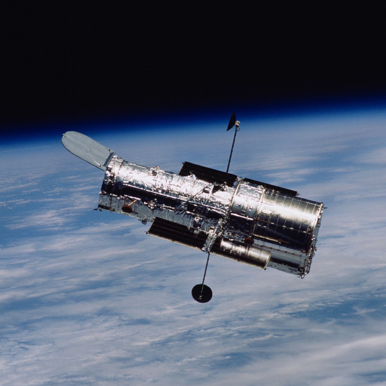
Hubble Space Telescope in orbit above Earth, as shown in the paper's instrument figure.

The reference · from space

Hubble Space Telescope

F814W images provide the higher-resolution target. Weight maps and source catalogues support reliable training and evaluation.

Reference band
ACS / F814W
Target cutout
256² at ×2 · 512² at ×4

HST is an observational reference, not an artifact-free image of the physical sky. Photo: NASA, reproduced in the paper.

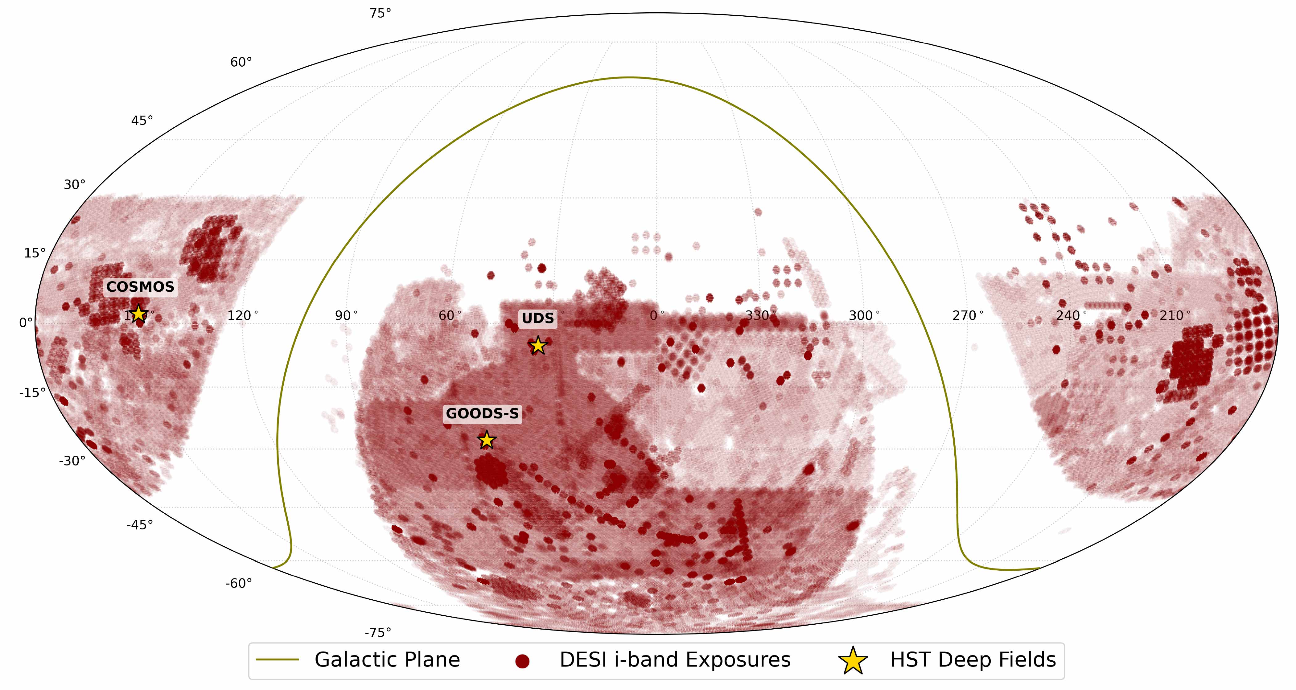
Where the observations meetView full figure ↗
Paper survey overview: DESI i-band sky coverage, Galactic plane, and the labelled HST deep fields COSMOS, UDS and GOODS-S.
DESI i-band coverage (red) and HST deep fields (gold). This paper figure shows survey coverage; the prepared split below contains COSMOS and UDS samples.

The research

Abstract

Useful detail, supported by measured light

FluxFlow is a conditional flow-matching model for astronomical image super-resolution. It learns in pixel space from real paired DESI–HST observations, using uncertainty maps and source-region weights to guide training.

During inference, measurement-consistent flow sampling (MC-FS) uses a Wiener-regularized correction to bring generated detail toward agreement with the measured input. This addresses a central generative-model risk: source-like structures unsupported by the observation.

Experiments evaluate image structure, source flux and downstream measurements at ×2 and ×4. Reconstructed images remain estimates; measurement consistency reduces the risk of unsupported sources but does not establish that every faint source is real.
The dataset

Learning from real image pairs

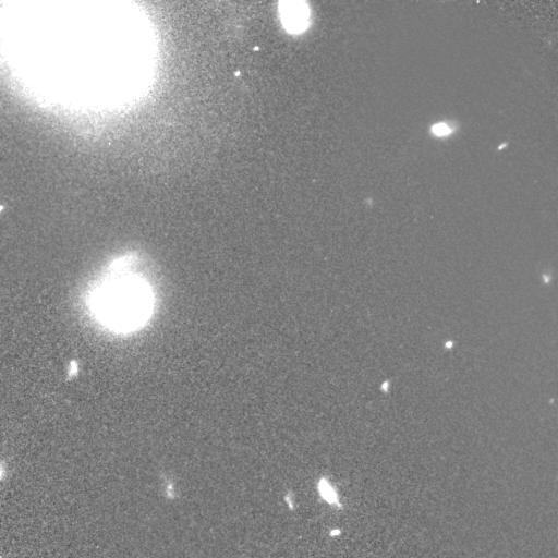
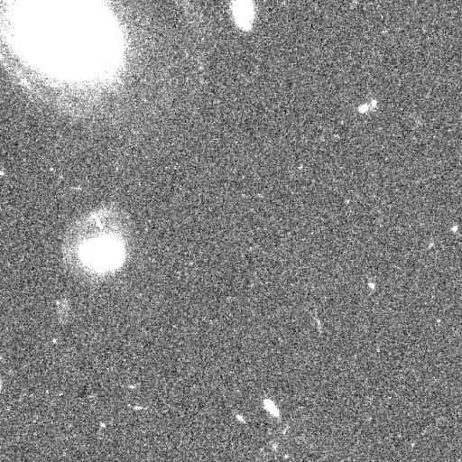
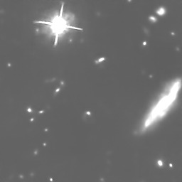
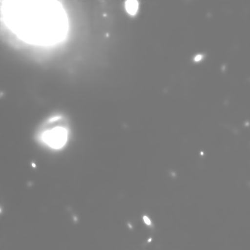
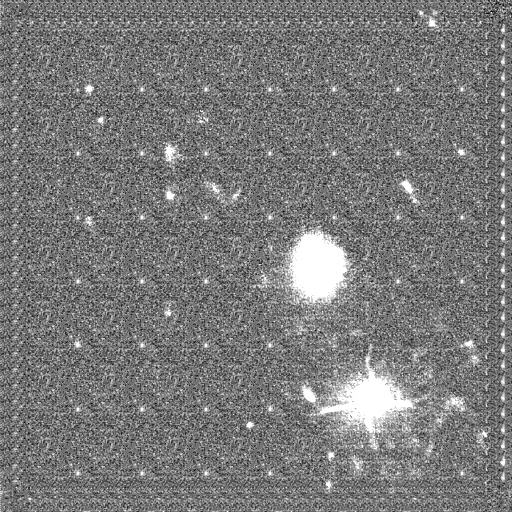
Real DESI–HST pairs let us compare the input, reconstruction and reference at the same sky position.

Prepared pairs / scale
19,438
Training pairs
17,737
Test pairs
1,701
Target scales
×2 / ×4
Input → reconstruction → referencePaired examples from the paper

Swipe through the same field — tap an image to inspect it

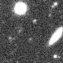
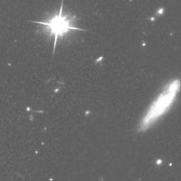
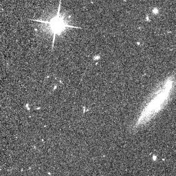
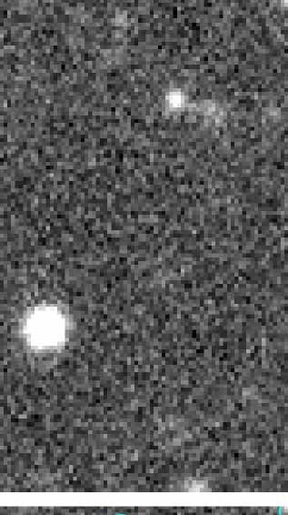
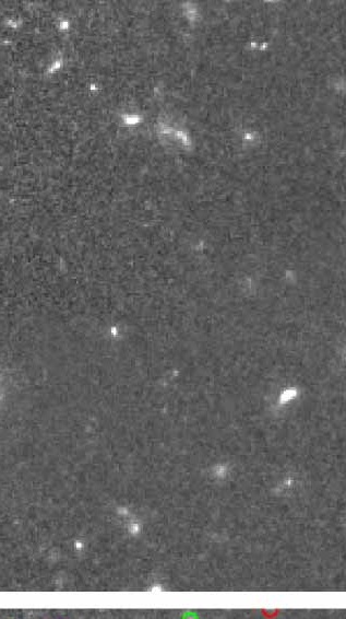
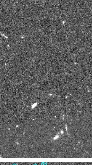
DESI inputFluxFlow reconstructionHST reference

DESI input

Field A ground observation at 128 by 128.128 × 128

FluxFlow reconstruction

Field A FluxFlow x2 reconstruction.×2 · 256 × 256

HST reference

Field A paired HST x2 reference.×2 · 256 × 256
DESI input · 1 of 3
Each scale shows a different example field; the three images within a panel are paired. The paper’s display scaling is preserved, so displayed brightness is not a calibrated measurement.

More than image pairs HST weight maps describe measurement reliability; source labels and catalogues support source-level evaluation.

Counting the data The paper describes approximately 19,500 pairs. The prepared split has 19,438 pairs per scale from COSMOS and UDS. The ×2 and ×4 versions share sample identities.

Data fields and evaluation context
  • desi_sci.npyi-band ground observation
  • hst_sci.npyHST observational reference
  • hst_wht.npyInverse-variance weights
  • hst_masks.npySource labels
  • hst_sources.npzSource catalogue

The historical patch-level split contains overlapping sky regions between training and test samples. It supports comparison under that protocol; it should not be described as a spatially independent generalization test.

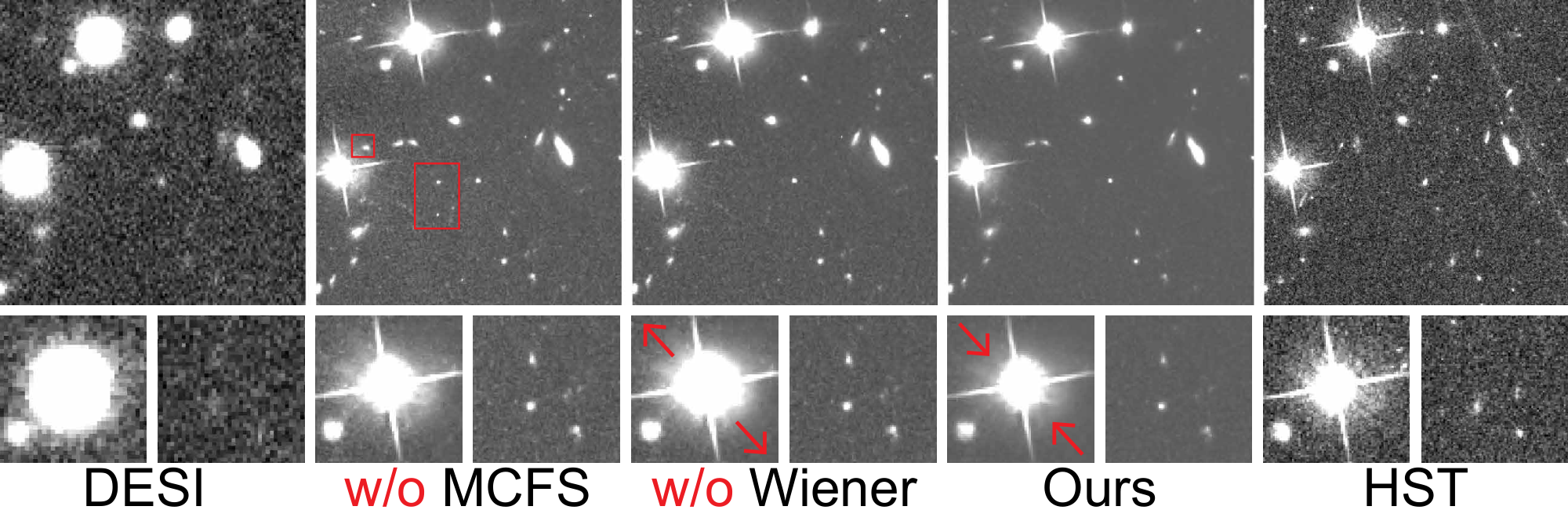
What happens without the correction?Inspect full figure ↗

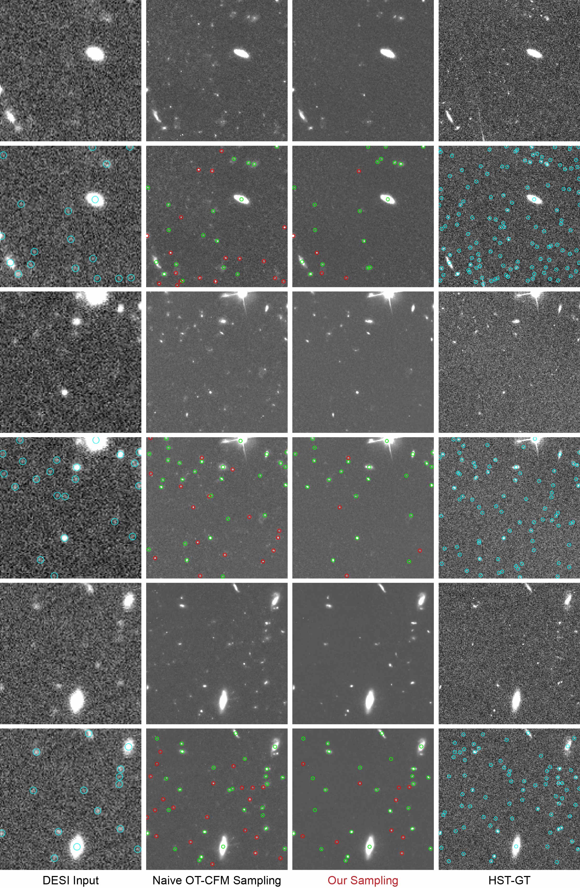
Start with the red boxesCompare the boxed spots in “w/o MCFS” with HST, then inspect the full method in “Ours”

Original MC-FS ablation figure: DESI, without MC-FS, without Wiener correction, FluxFlow and HST. Red boxes mark example unsupported sources.
Original paper ablation — red boxes mark example unsupported structures. The figure also compares removal of the Wiener correction with the full method and HST.

The challenge

Is that faint source really there?

Generative detail can look convincing even when the observation does not support it.

The riskA model can turn a noise fluctuation into a plausible-looking star or galaxy, producing an unreliable source catalogue.

The checkBlur and downsample the reconstruction, then compare it with DESI. MC-FS uses this discrepancy to reduce unsupported structure.

The limitAgreement with the input reduces this risk. It cannot establish that every reconstructed faint source is real.
The method

Reconstructing with measured light

Learn an update in pixel space, then check the reconstruction against the measured light.

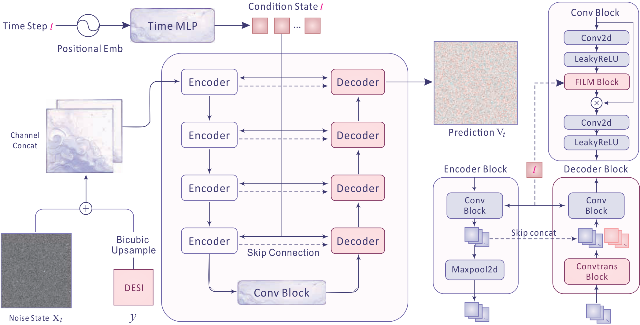
01 DESI + noise state02 Encoder–decoder03 Velocity prediction

View the whole model — switch to details to read its layers

Time-conditioned U-Net · complete architectureOpen original figure ↗PDF ↗

1Learn in pixel space

A time-conditioned U-Net learns to move Gaussian noise toward an HST-style image, with DESI as the observation condition.

2Weight reliable evidence

During training, square-root WHT weights and HST-derived source masks emphasize reliable pixels and scientifically useful structure.

3Apply measurement consistency

At each sampling step, a Gaussian-PSF and downsampling model predicts the ground observation. A Wiener-regularized correction reduces the residual.

The architecture is the original paper figure. The three animations explain training and sampling; they are schematics rather than recorded intermediate states.

The evidence

Preserving light and structure

Lower Flux-L1 indicates less source-flux error; higher SSIM indicates greater structural similarity.

Super-resolution scale

DESI–HSTSource-level Flux-L1Paper Table 2

Flux-L1 · ×2

2.959

Lowest Flux-L1 in the reported comparison

×2 · lower is better
Source-level flux error

Structural similarity · SSIM0.714

SSIM · ×2
SwinIR 0.702FluxFlow 0.714
SSIM · ×4
SwinIR 0.569FluxFlow 0.570
Flux-L1 · ×4
FISR 4.082FluxFlow 3.755

FluxFlow achieves the lowest Flux-L1 in the reported comparison at both scales. The complete table retains all reported metrics and baselines.

Quantitative evidenceFull comparison table

Complete reported comparisonPaper · Table 2

Explore the results

Compare the reconstructions

Choose a field and method, then move the divider to inspect the same region in both reconstructions.

Read structure, then check the referenceInspect source shapes and diffraction patterns. The HST option shows the paired observation; displayed brightness is not a flux measurement.

Super-resolution

×2

128² → 256² pixels
HATFluxFlow
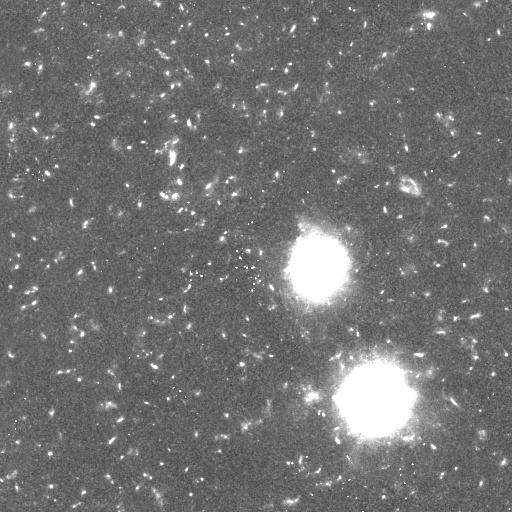
HAT result for Field A at x2FluxFlow result for the same Field A at x2

Field A · ×2 · HAT vs FluxFlow

Drag to compare · Arrow keys also work

Super-resolution

×4

128² → 512² pixels
HATFluxFlow
HAT result for Field D at x4FluxFlow result for the same Field D at x4

Field D · ×4 · HAT vs FluxFlow

Drag to compare · Arrow keys also work

Missing methods are disabled for that field. HST is an observational reference; no substitute images are used.

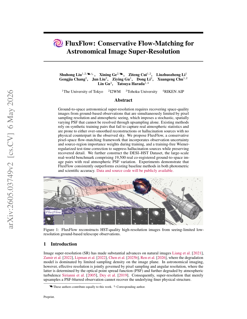
First page of the FluxFlow arXiv paper, version 2.
FluxFlow · arXiv paper, v2

Paper and citation

Paper and resources

FluxFlow: Conservative Flow-Matching for Astronomical Image Super-Resolution

arXiv:2605.03749 · 2026

Citation
@misc{liu2026fluxflow,
  title = {FluxFlow: Conservative Flow-Matching for Astronomical Image Super-Resolution},
  author = {Liu, Shuhong and Ge, Xining and Xu, Quanfeng and Cui, Ziteng and Li, Liuzhuozheng and Chang, Gengjia and Liu, Jun and Gu, Ziying and Li, Dong and Chu, Xuangeng and Gu, Lin and Harada, Tatsuya},
  year = {2026},
  eprint = {2605.03749},
  archivePrefix = {arXiv},
  primaryClass = {cs.CV},
  url = {https://arxiv.org/abs/2605.03749}
}

Interactive explanationSampling and implementation

Overview

Observe — reconstruct — check

A conservative flow learns the structure. A measurement-consistent correction keeps it grounded in the observation.

Ground observation yConditioning + uncertainty weights
01 / Initialise

Gaussian noise

x⁰ ~ N(0, I)

02 / Transport

Conservative flow

Short, straight-path ODE

03 / Correct

MC-FS

Wiener residual correction

04 / Reconstruct

Recovered field

Structure + integrated flux

Forward projection A = DₛHPSFResidual against observation y
The framework Condition on the DESI frame, transport along the learned flow, then correct the forward-model residual at each sampling step.

THE SAMPLER

A field unfolds — one step at a time

Ground observation
Complete DESI observation of the same field Complete FluxFlow reconstruction, progressively revealed by scrolling
DESI → FluxFlow 0%Full sampling figure ↗

The sampler, step by step

  1. Ground observationDESI, seeing-limited. The PSF has already destroyed the high-frequency content, and read noise sits on top of it.
  2. Flow transportThe state starts as pure noise, x⁰ ~ N(0, I). A conditional U-Net carries it along the straight-path interpolant with Euler steps.
  3. Forward projectionThe estimate is pushed back through the forward model A = DsHPSF — a Gaussian PSF of width σPSF = 2, then area downsampling — and the residual against the DESI frame is formed.
  4. Wiener correctionThe residual is Wiener-deconvolved with λSNR = 50 and subtracted, scaled by ηi = η0(1 − i/N). This is what holds hallucinations out.

Scroll to step through the sampler.

The technical notesInside the sampler ↗

08AInside the sampler

The flow and its mechanics

Measurement-consistent flow sampling. The velocity network proposes; the forward model disposes. Every step is projected back onto the observation — which is what keeps hallucinated sources out of the estimate.

  1. Illustrative thumbnail; the actual initial state is pure Gaussian noise1Noisy state xtx⁰ ~ N(0, I)
  2. the second field2DESI observation ybicubic → HR grid
  3. one field, two resolutions3Conditional U-Net vθpixel space · base_dim = 48 · FiLM time conditioning, 256-d
  4. bicubic reference4Euler stepx̃ = x + vθ Δt
  5. HAT baseline5Forward projectionA = DsHPSF, σPSF = 2
  6. FluxFlow output6Wiener correctionW(k) = H*(k)/(|H(k)|² + λSNR−1) · residual r = A(x̃) − y
  7. the recovered field7Corrected estimatex ← x̃ − ηi F−1(W F[Ds⊤r])

The thumbnails are illustrative stand-ins, not the sampler’s actual intermediate states — step 1 starts from pure Gaussian noise, and the correction runs on residuals, not on Bicubic or HAT images.

01 · Weight the evidence

wp = √Wp · (1 + Mp)

  • Wpinverse-variance weight (hst_wht)
  • Mpsource mask, from source detection on the HST truth image

Per-image loss normalised by the sum of pixel weights · Eq. 5, paper §5.1 · hst_wht.npy, hst_masks.npy

02 · Correct without retraining

W(k) = H*(k)|H(k)|2 + λSNR−1

  • Training-freeback-projection, not a network
  • Residualthrough the forward operator

Eq. (10) in the paper · removes sources the observation never had

03 · Settings as reported

Euler steps
N = 10
Base step
η0 = 0.5
Regularisation
λSNR = 50
PSF width
σPSF = 2

ηi = η0 (1 − i/N) · optimum 1.92, rounded

04 · Ablation · weight term removed

PSNR
31.2330.17
SSIM
0.7140.685
Precision
0.7380.688
F1
0.54120.5272

Full model → w/o WHT · paper Table 3

05 · Algorithm 1 · MC-FS

Algorithm 1  MC-FS
  inputs   observation y, PSF h, steps N, base step eta_0
  steps    t_i = i / N,   dt = 1 / N
  precompute  W(k) from Eq. (10)
  x <- x0 ~ N(0, I)
  for i = 0 .. N-1 do
    xt  <- x + v_theta(x, t_i, c) * dt     Euler step
    r   <- A(xt) - y                       residual to forward model
    eta_i <- eta_0 * (1 - i / N)           linear decay
    x   <- xt - eta_i * F^-1(W * F[Ds^T r]) Wiener-corrected update
  return x

The proposal is the network; the correction is the forward model.

Reproduce it
git clone https://github.com/I2WM/FluxFlow

# inference settings as reported in the paper
#   sampling steps            N        = 10 Euler steps
#   base correction step      eta_0    = 0.5      (eta_i = eta_0 (1 - i/N))
#   Wiener regularisation     lambda_SNR = 50
#   forward PSF width         sigma_PSF  = 2      (data-driven optimum 1.92, rounded)
#   correction mode           adjoint            --correction_mode adjoint swaps the Wiener
#                                                inverse for a plain adjoint
#   correction off            --no_mcfm          removes the correction entirely
#
# Check the repository README for the current command-line interface:
# https://github.com/I2WM/FluxFlow
The peopleAuthors & institutions

The research / The people

Authors and institutions

FluxFlow: Conservative Flow-Matching for Astronomical Image Super-Resolution.

Shuhong Liu1,2*◆· Xining Ge2*·Quanfeng Xu3*·Ziteng Cui1

Liuzhuozheng Li1· Gengjia Chang2· Jun Liu2· Ziying Gu1

Dong Li2· Xuangeng Chu1,2· Lin Gu4· Tatsuya Harada1,5

1The University of Tokyo 2I2WM 3Shanghai Astronomical Observatory (SHAO) 4Tohoku University 5RIKEN

* Equal contribution  ·  ◆ Corresponding author

Appendix Supplementary details Benchmark details, ablations, downstream measurements and implementation. Expand a topic to explore the evidence.
Appendix · ablations The four knobs that matter

Every hyper‑parameter of MC‑FS is swept in the appendix, over the paper’s own ranges (T = 5–60 steps, η0 = 0.1–1.0). The curves are trend schematics only — hand‑drawn to match the reported shapes and optima of Figs. 18–21, not measured data. The vertical axis is a schematic 0–1 scale, and the curves must not be used for numerical comparison.

Forward PSF width σPSF

2.0

Default σPSF = 2 HR pixels at both scales.

Wiener regularisation λSNR

50

Default λSNR = 50, the value used throughout Table 2.

Base correction step η0

0.50

Default η0 = 0.5, with per‑step decay ηi = η0(1 − i/N).

Sampling steps T

10

Default T = 10, all other MC‑FS hyper‑parameters at their defaults.

  • Source prior. Replacing the Gaussian source with a bicubic bridge helps the velocity field locally but couples the prior too tightly to the bicubic mean, suppressing the high‑frequency content pixel‑space OT‑CFM recovers under MC‑FS guidance. The Gaussian source is retained.
  • Pixel space vs latent space. Compared with the full model in Table 3, the frozen SD‑VAE variant has worse PSNR, SSIM, Flux‑L1, recall and F1: −2.33 dB PSNR, −0.121 SSIM, and recall of 0.211. Precision is higher (0.859 vs 0.738), while F1 is lower (0.3402 vs 0.5412).
  • Scale of the study. The paper describes approximately 19,500 DESI–HST pairs. The prepared split contains 19,438 pairs per scale, evaluated at ×2 and ×4.
Caption wording these curves are drawn from
  • Fig. 18 — “PSNR decreases monotonically with σPSF, while Flux‑L1 and Detection F1 form broad plateaus over an intermediate range. We set σPSF = 2 HR pixels at both scales.”
  • Fig. 19 — “Sweeping λSNR from 10 to 100 leaves PSNR, Flux‑L1, and Detection F1 essentially unchanged, in agreement with the spectral analysis of Sections E.2 and E.3.”
  • Fig. 20 — “PSNR is concave with a peak near η0 ≈ 0.4, Flux‑L1 grows monotonically, and Detection F1 peaks near η0 ≈ 0.3 before falling.”
  • Fig. 21 — “PSNR decreases monotonically with T; Flux‑L1 and Detection F1 attain their joint optimum at T = 10 before degrading at larger T as the per‑step Wiener correction ηi shrinks faster than the cumulative ODE drift along vθ.”
Appendix H · downstream science Does it change the science?

Photometric metrics are a proxy. The real question is whether a reconstruction makes the catalogue measurements better. Every number below is measured on the matched bright‑source set, under the same SEP segmentation footprint as the ground truth, with one common threshold Fthr = 0.5 nMgy at both scales.

Lower is better in every column. Magnitude and shear are dimensionless; stellar‑mass MAE is in Θ★‑scaled nanomaggies.

Per‑source downstream accuracy on the matched bright‑source set (paper Tables 8 and 9).
Method Magnitude residual Δm Stellar‑mass MAE Shear residual
meanmedian meanmedian meanmedian
Bicubic0.7580.6377.7671.5370.1480.122
SwinIR0.6490.3008.1970.7620.1490.116
HAT0.5420.1927.9620.5240.1510.112
FISR0.5610.2308.0140.6080.1650.133
cGAN0.5480.2157.9960.5860.1590.131
GD‑Net0.6640.3937.6591.0250.1660.131
FluxFlow0.5160.1877.6320.5080.1610.126

What improves. FluxFlow returns the lowest magnitude residual and the lowest stellar‑mass MAE — on both the mean and the median, at both scales. At ×4 the mean magnitude residual improves from 0.876 (FISR, best baseline) to 0.851, and the mean mass MAE from 16.19 (HAT, best baseline) to 16.07 Θ★‑scaled nanomaggies.

What does not. Shear is the flat metric. It is set by the second‑moment tensor of each source, and its orthogonal failure mode is catalog‑level miscentering rather than image quality, so the ranking compresses and the strongest baseline depends on scale and statistic: at ×4 HAT leads both shear mean (0.108) and median (0.081); at ×2 the shear mean is lowest for Bicubic (0.148) and the median for HAT (0.112). FluxFlow lands just behind the leader rather than ahead.

Why the mass median is the headline. The median stellar‑mass MAE is where bright, cleanly segmented sources live; the mean is dragged by a handful of blended or badly segmented objects, which is why GD‑Net posts a competitive mean (7.659) but a median of 1.025.

Appendix A & F · the benchmark The paired-image benchmark

DESI–HST is a cross‑survey benchmark: ground‑based seeing‑limited spectra‑era imaging on one side, space‑based diffraction‑limited imaging on the other. Reddy et al. 2024 is also G→S in that table, but without flux calibration and at 2,880 pairs — this set is the only one there combining real data, absolute flux calibration and the ground‑to‑space direction, and the largest real G→S set in it.

DESI · seeing‑limited 1.0–1.3″ FWHM
HST · diffraction‑limited ~0.09″ FWHM

The resolution gap is dominated by atmospheric turbulence, not by pixel scale: a 11–14× ratio in FWHM (a 2.4 m space aperture against DESI's time-varying, spatially extended i‑band seeing). That is what makes DESI→HST super‑resolution substantially harder than benchmarks that rely on pixel‑scale downsampling alone.

Astronomical super‑resolution datasets (paper Table 1). ✓ marks real data and absolute flux calibration; the last column is the imaging direction.
DatasetSizeRealFluxType
Miao et al. 20242,000✓G→G
Shan et al. 20259,383✓G→G
Song et al. 20241,597✓S→G
Reddy et al. 20242,880✓G→S
Luo et al. 202517,000✓G→G
Li et al. 202214,604✓G→G
Wu et al. 202554,738✓✓S→S
Zhang et al. 2026120,000✓S→G
FluxFlow (ours)19,500✓✓G→S

G ground‑based imaging · S space‑based imaging · → the direction of the super‑resolution mapping.

Supervised on other benchmarks

The same architecture, with the terms that need flux calibration switched off — the inverse‑variance term, the source‑importance term and the Wiener‑deconvolved measurement consistency are not available on these sets, so an ablated configuration is evaluated instead.

  • STAR at ×2 — highest PSNR and SSIM, together with a top‑tier Flux‑L1.
  • STAR at ×4 — remains competitive with the strongest regression baselines.
  • AstroSR at ×2 — highest PSNR and a competitive SSIM.

The honest caveat. AstroSR is distributed as RGB composites without absolute flux calibration, so total brightness is no longer conserved across the SDSS→HSC mapping. The Flux‑L1 column on that benchmark carries limited physical meaning and is reported only for completeness. The margins over regression baselines are markedly smaller than on DESI–HST, because neither dataset exposes super‑resolution under atmospheric aberration — the dominant degradation mode this method is built for is simply absent.

Appendix E · analysis Why the adjoint is not enough
  1. E.1

    The consistency set

    A source whose morphology has no preimage under A still produces a non‑zero forward residual, so it is penalised wherever the correction enforces y = A(x). Hallucinations are therefore not undetectable in principle — they are trajectories that exit the consistency set C(y), and the whole sampler is built to push them back in.

  2. E.2

    The Wiener kernel from MMSE

    Minimising the mean‑square error over the Fourier‑domain filter, setting the variation to zero and solving gives the optimal filter W(k) = H*(k) / (|H(k)|² + λSNR−1).

  3. E.3

    Spectral analysis

    Naive adjoint back‑projection contracts high‑frequency modes at a rate of |H(k)|² per step, so the loss accumulates into PSF‑scale smoothing across integration steps. Replacing that multiplier with the Wiener kernel keeps the cumulative transfer function stable at high frequencies and preserves the resolution gain the flow provides.

  4. E.4

    Closed‑form toy model

    A normalised 2‑D Gaussian PSF of width σh, probed with a single point source of amplitude α, restricted to the band the LR observation actually supports, iterated for N Euler steps — giving an exact per‑mode recovery factor rather than a fixed‑point approximation.

Two limits and their interpretation

λSNR → ∞

W(k) → H*(k)/|H(k)|² = 1/H(k)

The exact inverse filter. Maximally amplifies high frequencies and is unstable wherever H(k) ≈ 0.

λSNR → 0

W(k) → λSNR H*(k) → 0

The response stays proportional to the matched filter — equivalent, up to scaling, to the raw adjoint. This is exactly the variant the ablation calls w/o Wiener.

λSNR therefore interpolates continuously between the two extremes, and controls how aggressively the deconvolution restores the high‑frequency content the PSF suppressed.

Recovered profile width — FWHM in HR pixels

True PSF 4.71
Naive adjoint · N = 10 6.78
Wiener‑corrected 4.85

At N = 10 the naive recovery is visibly broader than the true PSF — the FWHM is enlarged from 4.71 to 6.78 HR pixels, while the Wiener‑corrected profile comes in at 4.85 and tracks the true PSF with in‑line width. The widening is a low‑pass effect, not noise amplification.

The honest caveat, in the paper's own analysis. If the iteration were run to convergence instead of a finite N, the fixed‑point per‑pixel variance evaluates to roughly 0.21 σ²n at the DESI–HST setting (σh = 2, kmax = π/4). Modest in absolute terms, but it is a substantial amplification of the noise power inside the narrow LR‑supported band, and the prefactor grows exponentially as kmax approaches Nyquist. The practical N = 10 keeps the recovery short of that fixed point — so in this regime the dominant pathology is the finite‑N low‑pass effect of Eq. 27, not the asymptotic noise amplification of Eq. 30.

Table 3 · ablation What each piece is worth
Ablation on photometry and detection metrics (paper Table 3). WHT = inverse‑variance weighting, Src = source‑weighted loss.
Ablation Photometry Detection
PSNR ↑SSIM ↑Flux‑L1 ↓ Prec ↑Rec ↑F1 ↑
w/ VAE28.900.5935.0750.8590.2110.3402
w/ Bridge30.770.6633.2060.7020.3930.5019
w/o WHT30.170.6852.8140.6880.4830.5272
w/o Src31.160.7113.0980.7290.4640.5382
w/o MC‑FS30.780.6983.0250.6020.5530.5256
w/o Wiener30.790.6993.0310.7080.4480.5066
Ours31.230.7142.9590.7380.4580.5412

The one that matters most. Without MC‑FS the sampler produces compact hallucination sources, and the table shows the signature: the highest recall in the whole study (0.553) together with a precision collapse to 0.602. The spurious peaks float as false positives and drag F1 to 0.5256, below the full model's 0.5412.

The quiet trade‑off. w/o WHT posts a marginally better Flux‑L1 (2.814 vs 2.959) — and that is reported rather than hidden, because it comes from fitting drizzle artefacts that overlap the source apertures. Without the WHT term the velocity field treats cosmic‑ray trails and chip gaps as valid targets and reproduces them in the reconstruction; the drops in PSNR, F1 and precision are the real cost.

Source weighting. A uniform loss is dominated by background pixels and cannot preferentially preserve the faint outer galaxy profiles that carry morphological and PSF‑shape information. The two weights are complementary: WHT filters data quality, source weighting emphasises scientifically informative regions.

Latent space. Moving the flow into a frozen SD‑VAE feature space costs 2.33 dB of PSNR and 0.121 of SSIM, and collapses recall to 0.211; the bridge variant that replaces the Gaussian source with a noisy bicubic mean recovers most of the photometry but still trails the full model on precision and F1.

Tables 6 & 7 · other benchmarks The same model on data it was not built for
STAR dataset (paper Table 6) at ×2 and ×4. PSNR / SSIM higher is better; Flux‑L1 lower is better. Best per row in bold-ish; FluxFlow highlighted.
ScaleMetric Method
BicubicEDSRSRGANRCANSwinIRHATFISROurs
×2PSNR ↑28.7133.5032.2533.8934.0534.3834.4034.66
×2SSIM ↑0.69450.77290.75010.78080.78120.78360.78590.7918
×2Flux‑L1 ↓125.448.7851.3543.4442.4141.2741.0541.84
×4PSNR ↑26.2130.7330.3332.1332.2432.6732.5132.44
×4SSIM ↑0.59930.65490.65220.68380.68810.69360.68910.6867
×4Flux‑L1 ↓239.267.4774.7260.5255.3548.4950.9457.20
AstroSR dataset (paper Table 7) at ×2.
ScaleMetric Method
BicubicEDSRSRGANRCANENLCASwinIRHATFISROurs
×2PSNR ↑17.7523.7123.4623.7223.7023.7423.8123.8423.87
×2SSIM ↑0.1710.3500.3480.3510.3500.3520.3520.3540.352
×2Flux‑L1 ↓1916213.6165.9226.3216.1223.1193.3192.5198.7

Read this column with care. AstroSR is distributed as RGB composites without absolute flux calibration, so total brightness is not conserved across the SDSS→HSC mapping: its Flux‑L1 column carries limited physical meaning and is reported only for completeness.

What it wins. On STAR at ×2 the model takes the highest PSNR (34.66) and the highest SSIM (0.7918), with a top‑tier Flux‑L1 (41.84, behind FISR's 41.05 and HAT's 41.27). At ×4 it stays competitive with the strongest regression baselines — HAT leads PSNR at 32.67 against 32.44. On AstroSR at ×2 it takes the highest PSNR (23.87) and a competitive SSIM (0.352 against FISR's 0.354).

Table 5 · training cost What it costs to train

×2 scale

SwinIR94 h
HAT552 h
FISR94 h
cGAN8 h
GD‑Net5 h
AS‑Bridge144 h
FluxFlow16 h

×4 scale

SwinIR98 h
HAT549 h
FISR176 h
cGAN16 h
GD‑Net184 h
AS‑Bridge360 h
FluxFlow47 h

Reading it. FluxFlow trains in 16 h at ×2 and 47 h at ×4 — 2.90% and 8.56% of the cost of the strongest Transformer regression baseline (HAT, 552 h / 549 h) respectively, and at ×4 about 7.7× faster than the heaviest generative baseline (AS‑Bridge, 360 h). Only the two cheapest baselines, cGAN and GD‑Net, train faster at ×2.

Appendix D · implementation How it is built
DESI observationbicubic → HR grid
&plus;
Noisy state xtGaussian source
EncoderConvBlock → 2×2 max‑pool, base_dim = 48, channels double per level
BottleneckConvBlocks at the lowest resolution
DecoderConvTransBlock upsampling &plus; skip connections from the matching level
Velocity vθpredicted on the HR grid

Every ConvBlock is Conv2d → LeakyReLU → FiLM → Conv2d → LeakyReLU. The FiLM layer applies a feature‑wise affine modulation conditioned on the time‑conditioning state τ, so the time signal is injected at every resolution rather than only at the input. The timestep t ∈ [0,1] is mapped to τ by a sinusoidal positional embedding followed by a two‑layer MLP of output dimension 256.

Training

Objective
OT‑CFM, spatially weighted MSE (Eq. 5)
Interpolant
xt = (1−t)x0 + t x1, target ut = x1 − x0
Sampling
x0 ~ N(0, I), t ~ U(0,1)
Grad clipping
1.0
Schedule
1,000‑step linear warm‑up → cosine decay to zero
Precision
fp32
EMA eval
every 20 epochs, 10 Euler steps from pure Gaussian noise

Normalisation

Clip thresholds
0.01% tail percentiles of all training‑split pixels
Why
suppresses cosmic rays and hot pixels that would otherwise set the range
Thresholds
one pair for the LR set, another for the HR set — estimated once, then frozen
Rescaling
linear min–max to [0,1] using global per‑modality flux extrema
Reporting
PSNR / SSIM are measured in that normalised domain, so the maximal value is exactly 1

Forward‑model PSF

Calibration
γPSF swept on a fine grid; the minimising value is rounded to an integer
Result
data-driven optimum σ* = 1.92, rounded to σPSF = 2 HR pixels and used throughout inference
Cross‑check
consistent with the median DECam i‑band seeing in Appendix A

Cost

Hardware
single NVIDIA A100‑80GB, identical schedule budget for all baselines
×2 scale
16 h end‑to‑end training
×4 scale
47 h end‑to‑end training
Appendix I · additional visualisation What to look for in the comparisons
  1. Figure 24 · ×2

    FluxFlow recovers the diffraction spikes of the central star and the morphology of the extended source, while avoiding the speckled background of AS‑Bridge.

  2. Figure 25 · ×2

    On a bright central star surrounded by closely packed compact sources, FluxFlow reproduces the spike pattern and resolves the neighbouring sources without the merging or smearing seen in the baselines.

  3. Figure 26 · ×4

    On a field with a saturated source in the upper‑left corner and several low‑SNR background galaxies, FluxFlow preserves faint background galaxies that Bicubic and GD‑Net erase, while reconstructing the saturated halo more cleanly than the speckled output of AS‑Bridge.

  4. Figure 27 · ×4

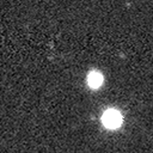
    On a binary‑star field, FluxFlow reproduces the four‑pointed diffraction pattern on the lower companion together with surrounding faint sources — whereas regression baselines suppress the spike pattern and the generative baselines either over‑smooth or over‑sharpen the background.

The panels in the comparison gallery above are real cut‑outs sliced from the paper's own comparison grids — every one of the 42 tiles is a genuine render, not a reconstruction of one.

Open original ↗